Computing Eigenvalues of 2x2 Matrices
This is a video for anyone who already knows what eigenvalues and eigenvectors are, and who might enjoy a quick way to compute them in the case of 2x2 matrices. As a quick reminder, if the effect of a linear transformation on a given vector is to scale it by some constant, we call it an “eigenvector” of the transformation, and we call the relevant scaling factor the corresponding “eigenvalue,” often denoted with the letter lambda.
To find the eigenvalues, there are only three relevant facts you need to know:
- The trace of a matrix, which is the sum of the two diagonal entries, is equal to the sum of the eigenvalues.
- The determinant of a matrix is equal to the product of the two eigenvalues.
- The two eigenvalues are evenly spaced around the mean of the two diagonal entries, and the distance between them can be found from the product of the two eigenvalues.
In other words, the two eigenvalues for a 2x2 matrix can be found from the following formula:
$$\lambda_1, \lambda_2 = \frac{Trace \pm \sqrt{Trace^2 - 4 Det}}{2}$$ For any mean, $m$, and product, $p$, the distance squared is always going to be $m^2 - p$. This gives the third key fact, which is that when two numbers have a mean $m$ and a product $p$, you can write those two numbers as $m \pm \sqrt{m^2 - p}$. This is decently fast to rederive on the fly if you ever forget it, and it’s essentially just a rephrasing of the difference of squares formula. But even still it’s a fact worth memorizing so that you have it at the tip of your fingers. In fact, my friend Tim from the channel acapellascience wrote us a quick jingle to make it a little more memorable.
m plus or minus squaaaare root of me squared minus p (ping!)
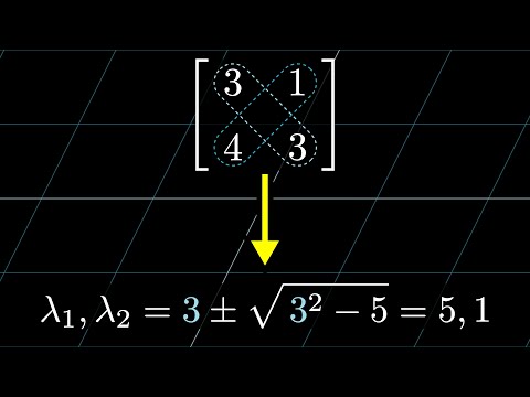
Let me show you how this works, say for the matrix [[3,1], [4,1]]. You start by bringing to mind the formula, maybe stating it all in your head. But when you write it down, you fill in the appropriate values of $m$ and $p$ as you go. So in this example, the mean of the eigenvalues is the same as the mean of 3 and 1, which is 2. So the thing you start writing is $2 \pm \sqrt{2^2 - \dots}$. Then the product of the eigenvalues is the determinant, which in this example is $3 \times 1 - 1 \times 4$, or -1. So that’s the final thing you fill in. This means the eigenvalues are $2 \pm \sqrt{5}$. You might recognize that this is the same matrix I was using at the beginning, but notice how much more directly we can get at the answer.
Here, try another one. This time the mean of the eigenvalues is the same as the mean of 2 and 8, which is 5. So again, you start writing out the formula but this time writing 5 in place of $m$. And then the determinant is $2 \times 8 - 7 \times 1$, or 9. So in this example, the eigenvalues look like $5 \pm \sqrt{16}$, which simplifies even further as 9 and 1. You see what I mean about how you can basically just start writing down the eigenvalues while staring at the matrix? It’s typically just the tiniest bit of simplifying at the end.
Honestly, I’ve found myself using this trick a lot when I’m sketching quick notes related to linear algebra and want to use small matrices as examples. I’ve been working on a video about matrix exponents, where eigenvalues pop up a lot, and I realized it’s just very handy if students can read off the eigenvalues from small examples without losing the main line of thought by getting bogged down in a different calculation.
As another fun example, take a look at this set of three different matrices, which come up a lot in quantum mechanics, they’re known as the Pauli spin matrices. If you know quantum mechanics, you’ll know that the eigenvalues of matrices are highly relevant to the physics they describe, and if you don’t know quantum mechanics, let this just be a little glimpse of how these computations are actually relevant to real applications.
The mean of the diagonal in all three cases is 0, so the mean of the eigenvalues in all cases is 0, which makes our formula look especially simple. What about the products of the eigenvalues, the determinants of these matrices? For the first one, it’s 0 - 1 or -1. The second also looks like 0 - 1, but it takes a moment more to see because of the complex numbers. And the final one looks like -1 - 0. So in all cases, the eigenvalues simplify to be ±1. Although in this case, you really don’t need the formula to find two values if you know they’re evenly spaced around 0 and their product is -1.
If you’re curious, in the context of quantum mechanics, these matrices describe observations you might make about a particle’s spin in the x, y or z directions. The fact that their eigenvalues are ±1 corresponds with the idea that the values for the spin that you would observe would be either entirely in one direction or entirely in another, as opposed to something continuously ranging in between. Maybe you’d wonder It’s funny that I wrote this section because I wanted to show examples of 2x2 matrices that come up in practice, and quantum mechanics is great for that. However, I realized that this example actually undercuts the point I’m trying to make. For these specific matrices, it’s essentially just as fast to use the traditional method with characteristic polynomials, and it might even be faster.
Where you will actually feel the speed up is in the more general case where you take a linear combination of these three matrices and try to compute the eigenvalues. This would describe spin observations in a general direction of a vector with coordinates [a, b, c], where you should assume the vector is normalized, meaning a^2 + b^2 + c^2 = 1. With this new matrix, it’s immediate to see that the mean of the eigenvalues is still zero, and the product of those eigenvalues is still -1.
The real advantage of using the mean-product formula is that it’s fewer symbols to memorize, and each one of them carries more meaning with it. You don’t need to go through the intermediate step of setting up the characteristic polynomial, but you can jump straight to writing down the roots without ever explicitly thinking about what the polynomial looks like. This is a very specific trick, but it’s something I wish I knew in college, so if you know any students who might benefit from it, consider sharing it with them. The hope is that it’s not just one more thing to memorize, but that the framing reinforces some other nice facts worth knowing, like how the trace and determinant relate to eigenvalues. If you want to prove those facts, by the way, take a moment to expand out the characteristic polynomial for a general matrix and think deeply about the meaning of each of these coefficients. Many thanks to Tim for making sure that this mean-product formula will remain in our minds for a few months. If you are not familiar with acapellascience, please do check it out. Especially worth mentioning is “The Molecular Shape of You”, which is one of the greatest things on the internet.