Now I’m going to tell you about a really nice puzzle involving the shadow of a cube. The point of this video is not about the puzzle itself, but about two distinct problem-solving styles that are reflected in two different ways that we can tackle this problem. To anthropomorphize these two different styles, let’s imagine two students, Alice and Bob, who embody each one of the approaches. Bob is the kind of student who loves calculation and as soon as he can dig into the details and get a concrete view of the situation in front of him, he’s pleased. Alice, on the other hand, prefers to get a nice high-level general overview of the problem she’s dealing with, the general shape that it has, before she digs into the computations. She’s most pleased if she understands the broader context of the question and if the general view can lead to more swift and elegant computations.
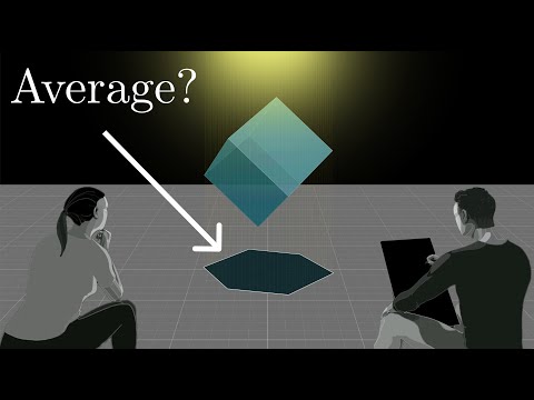
The puzzle they are faced with is to find the average area for the shadow of a cube. The size of the cube and its orientation influence the area of its shadow. The light source is assumed to be directly above the cube and infinitely far away, so that all we’re considering is a flat projection. For example, if the cube is straight up with two of its faces parallel to the ground, the shadow is a square and its area is the length of the side squared. Another special case is if the long diagonal is parallel to the direction of the light, in which case the shadow is a regular hexagon with an area equal to the square root of three times the area of one of the square faces.
The challenge is to find the average area over all possible orientations for a particular size of the cube. This also takes into account where the light source is, as it can distort the shadow and give it a different shape. So Bob’s thinking is that maybe the area of this shadow is some kind of function of theta that interpolates between those two values.
I think a lot of us have an intuitive feel for what we want it to mean, at least in the sense of what experiment would you do to verify it. You might imagine tossing this cube in the air like a die, freezing it at some arbitrary point, recording the area of the shadow from that position, and then repeating. If you do this many many times over and over you can take the mean of your sample. The number that we want to get at, the true average here, should be whatever that experimental mean approaches as you do more and more tosses approaching infinitely many. Even still, the sticklers among you could complain that doesn’t really answer the question, because it leaves open the issue of how we’re defining a “random” toss. The proper way to answer this, if we want it to be more formal, would be to first describe the space of all possible orientations, which mathematicians have actually given a fancy name. They call it SO(3), typically defined in terms of a certain family of 3-by-3 matrices. And the question we want to answer is “What probability distribution are we putting to this entire space?” It’s only when such a probability distribution is well-defined that we can answer a question involving an average. If you are a stickler for that kind of thing, I want you to hold off on that question until the end of the video. You’ll be surprised at how far we can get with the more heuristic experimental idea of just repeating a bunch of random tosses without really defining the distribution.
Once we see Alice and Bob’s solutions, it’s actually very interesting to ask how exactly each one of them defined this distribution along their way. And remember, this is not meant to be a lesson about cube shadows, per se, but a lesson about problem-solving told through the lens of two different mindsets that we might bring to the puzzle. And as with any lesson on problem-solving, the goal here is not to get to the answer as quickly as we can, but hopefully for you to feel like you found the answer yourself. So if ever there’s a point when you feel like you might have an idea, give yourself the freedom to pause and try to think it through. As a first step, and this is really independent of any particular problem-solving styles, just anytime you find a hard question, a good thing that you can do is ask “What’s the simplest possible non-trivial variant of the problem that you can try to solve?” In our case what you might say is, okay, let’s forget about averaging over all the orientations. That’s a tricky thing to think about. And let’s even forget about all the different faces of the cube, because they overlap and that’s also tricky to think about. Just for one particular face and one particular orientation, can we compute the area of this shadow? Once more, if you want to get your bearings with some special cases the easiest is when that face is parallel to the ground in which case the area of the shadow is the same as the area of the face. And on the other hand if we were to tilt that face 90-degrees, then its shadow will be a straight line and it has an area of zero.
So Bob looks at this and he wants an actual formula for that shadow, and the way he might think about it is to consider the normal vector perpendicular off of that face. What seems relevant is the angle that that normal vector makes with the vertical, with the direction where the light is coming from, which we might call theta. Now from the two special cases we just looked at, we know that when theta is equal to 0, the area of that shadow is the same as the area of the shape itself, which is s squared if the square has side lengths s. And if theta is equal to 90 degrees, then the area of that shadow is zero. So Bob’s thinking is that maybe the area of this shadow is some kind of function of theta that interpolates between those two values. It’s probably not too hard to guess that trigonometry will be somehow relevant, so anyone comfortable with their trig functions could probably hazard a guess as to what the right formula is. But Bob is more detail-oriented than that: he wants to properly prove what that area should be rather than just making a guess based on the endpoints.
The way you might think about it could be something like this: if we consider the plane that passes through the vertical as well as our normal vector, and then we consider all the different slices of our shape that are in that plane, or parallel to that plane, then we can focus our attention on a two-dimensional variant of the problem. If we just look at one of those slices, which has a normal vector an angle theta away from the vertical, its shadow might look something like this. And if we draw a vertical line up to the left here, we have ourselves a right triangle. And from here we can do a little bit of angle chasing, where we follow around what that angle theta implies about the rest of the diagram. And this means the lower right angle in this triangle is precisely theta.
So when we want to understand the size of this shadow in comparison to the original size of the piece, we can think about the cosine of that angle theta, which remember is the adjacent over the hypotenuse. It’s literally the ratio between the size of the shadow and the size of the slice. So the factor by which the slice gets squished down in this direction is exactly cosine of theta. And if we broaden our view to the entire square all the slices in that direction get scaled by the same factor. But in the other direction, the one perpendicular to that slice, there is no stretching or squishing because the face is not at all tilted in that direction. So overall the two-dimensional shadow of our two-dimensional face should also be scaled down by this factor of a cosine of theta.
It lines up with what you might intuitively guess given the case where the angle is 0 degrees and the case where it’s 90 degrees, but it’s reassuring to see why it’s true. Actually, as stated so far, this is not quite correct. There is a small problem with the formula that we’ve written. In the case where theta is bigger than 90 degrees, the cosine would actually come out to be negative, but of course we don’t want to consider the shadow to have negative area. At least not in a problem like this. So there’s two different ways you could solve this: you could say we only ever want to consider the normal vector that is pointing up, that has a positive z component. Or more simply we could say just take the absolute value of that cosine, and that gives us a valid formula.
So Bob’s happy because he has a precise formula describing the area of the shadow, but Alice starts to think about it a little bit differently. She says, okay we’ve got some shape, and then we apply a rotation that sort of situates it into 3D space in some way, and then we apply a flat projection that shoves that back into two-dimensional space. And what stands out to her is that both of these are linear transformations. That means that in principle you could describe each one of them with a matrix, and that the overall transformation would look like the product of those two matrices.
What Alice knows from one of her favorite subjects, linear algebra, is that if you take some shape and you consider its area, then you apply some linear transformation, the area of that output looks like some constant times the original area of the shape. More specifically we have a name for that constant, it’s called the determinant of the transformation. If you’re not so comfortable with linear algebra, we could give a much more intuitive description and say if you uniformly stretch the original shape in some direction, the output will also uniformly get stretched in some direction. Alice noted that the area of the shadow of any shape is proportional to the area of the original shape, and this proportionality constant does not depend on the size or shape of the original shape, but rather on the transformation being applied to it. Bob, on the other hand, is eager to compute this constant and will show us how in a few minutes. I do want to stay in Alice’s world for a little bit more, because this is where things start to really get fun. She is curious about how the area of the shadow of the cube relates to the area of its individual faces. She has the insight that if we think about the whole cube, not just a pair of faces, we can conclude that the area of the shadow for a given orientation is exactly one-half the sum of the areas of all of the faces. She justifies this by appealing to the idea of convexity, which states that a set is “convex” if the line that connects any two points inside that set is entirely contained within the set itself. This means that for our cube, because it is convex, between the first point of entry and the last point of exit it has to stay entirely inside the cube. So that’s the first key insight, the face shadows double-cover the cube shadow. And the next one is a little bit more symbolic, so let’s start things off by abbreviating our notation a little to make room on the screen. Instead of writing Area(Shadow(Cube)), I’m just going to write S(Cube). And similarly instead of Area(Shadow(a particular face)), I’m just going to write S(F_j), where that subscript j indicates which face I’m talking about. But of course, we should really be talking about the shadow of a particular rotation applied to the cube, so I might write this as S of some rotation applied to the cube. And likewise on the right, it’s the area of the shadow of that same rotation applied to a given one of the faces.
With the more compact notation at hand, let’s think about the average of this shadow area across many different rotations, some sample of R1, R2, R3, and so on. Again, that average just involves adding up all of those shadow areas and then dividing them by n, and in principle if we were to look at this for larger and larger samples, letting n approach infinity, that would give us the average area of the shadow of the cube.
Some of you might be thinking, “yes, we know this, you’ve said this already.” But it’s beneficial to write it out so that we can understand why it is that expressing the shadow area for a particular rotation of the cube as a sum across all of its faces, or one half times that sum at least…why is that beneficial? What is that going to do for us? Well, let’s just write it out, where for each one of these rotations of the cube we could break down that shadow as a sum across that same rotation applied across all of the faces. And when it’s written as a grid like this, we can get to Alice’s second insight, which is to shift the way that we’re thinking about the sum from going row-by-row to instead going column-by-column.
For example if we focused our attention just on the first column, what it’s telling us is to add up the area of the shadow of the first face across many different orientations. So if we were to take that sum and divide it by the size of our sample, that gives us an empirical average for the area of the shadow of this face. So if we take larger and larger samples, letting that size go to infinity, this will approach the average shadow area for a square. Likewise, the second column can be thought of as telling us the average area for the second face of the cube, which should of course be the same number. And same deal for any other column, it’s telling us the average area for a particular face.
So that gives us a very different way of thinking about our whole expression. Instead of saying add up the areas of the cubes at all the different orientations, we could say just add up the average shadows for the six different faces and multiply the total by one half. The term on the left here is thinking about adding up rows first, and the term on the right is thinking about adding up columns first.
In short, the average of the sum of the face shadows is the same as the sum of the average of the face shadows. Maybe that swap seems simple, maybe it doesn’t, but I can tell you that there is actually a little bit more than meets the eye to the step that we just took. But we’ll get to that later.
And remember, we know that the average area for a particular face looks like some universal proportionality constant times the area of that face, so if we’re adding this up across all the faces of the cube, we could think of this as equaling some constant times the surface area of the cube. And that’s pretty interesting, the average area for the shadow of this cube is going to be proportional to its surface area. Alice’s result is not obvious at first, as it’s not immediately clear that the average shadow area of a convex solid should be proportional to its surface area. However, the underlying assumption is that the probability distribution of all orientations should be uniform, meaning that the probability of any given patch of area on the sphere should be proportional to that area itself. Bob was able to use this to figure out that the area of a square’s shadow is only dependent on the cosine of the angle between the normal vector and the vertical. This is a neat result, as it allows us to avoid the extra degree of freedom that would arise from rotation about the normal vector. All those shadows are genuinely different shapes, but the area of each of them will be the same. This means that when Bob wants this average shadow area over all possible orientations, all he really needs to know is the average value of the absolute value of the cosine of theta for all different possible normal vectors. To compute an average like this, if we lived in a discrete, pixelated world, we would find the probability of landing on any particular value of theta, multiply it by the area of the shadow, and then add that up over all of the different possible values of theta ranging from 0 up to 180 degrees or pi radians. However, in reality there is a continuum of possible values of theta, and the probability of landing on any specific value is zero. To solve this, we compute an integral. To approximate an answer to this question without calculus, we take a sample of values for theta ranging from 0 up to 180 degrees. We then find the probability of falling between two different values from our sample, which is the area of the band divided by the total surface area of the sphere. The area of the band is approximately the circumference of the band (2πsinθ) times its thickness (Δθ). This is the key step.
What’s important is that for a finer sample of many more values of theta, the accuracy of the approximation would get better and better. Now remember, the reason we wanted this area was to know the probability of falling into that band, which is this area divided by the surface area of the sphere, which we know to be 4πr². That’s a value that you could also compute with an integral similar to the one that we’re setting up now, but for now we can take it as a given, as a standard well-known formula. And this probability itself is just a stepping stone in the direction of what we actually want, which is the average area for the shadow of a square. To get that we’ll multiply this probability times the corresponding shadow area, which is this absolute value of cosine theta expression we’ve seen many times up to this point. And our estimate for this average would now come down to adding up this expression across all of the different bands, all of the different samples of theta that we’ve taken.
This right here, by the way, is when Bob is just totally in his element. We’ve got a lot of exact formulas describing something very concrete, actually digging in on our way to a real answer. And again, if it feels like a lot of detail, I want you to appreciate that fact so that you can appreciate just how magical it is when Alice manages to somehow avoid all of this.
Anyway, looking back at our expression, let’s clean things up a little bit, like factoring out all of the terms that don’t depend on theta itself. And we can simplify that 2π/4π to simply be one half. And to make it a little more analogous to calculus with integrals, let me just swap the main terms inside the sum here. What we now have, this sum that’s going to approximate the answer to our question, is almost what an integral is. Instead of writing the sigma for sum, we write the integral symbol, this kind of elongated Leibnizian S showing us that we’re going from zero to pi. And instead of describing the step size as delta theta, a concrete finite amount, we instead describe it as “d” theta, which I like to think of as signaling the fact that some kind of limit is being taken.
What that integral means, by definition, is whatever the sum on the bottom approaches for finer and finer subdivisions, more dense samples that we might take for theta itself. And at this point, for those of you who do know calculus, I’ll just write down the details of how you would actually carry this out as you might see it written down in Bob’s notebook. It’s the usual anti-derivative stuff, but the one key step is to bring in a certain trig identity. In the end, what Bob finds after doing this is the surprisingly clean fact that the average area for a square’s shadow is precisely one-half the area of that square. This is the mystery constant which Alice doesn’t yet know. If Bob were to look over her shoulder and see the work that she’s done he could finish out the problem right now. He plugs in the constant that he just found and he knows the final answer.
And now, finally! With all of this as backdrop, what is it that Alice does to carry out the final solution? I introduced her as someone who really likes to generalize the results she finds. And usually those generalizations end up as interesting footnotes that aren’t really material for solving particular problems. But this is a case where the generalization itself draws her to a quantitative result. Remember, the substance of what she’s found so far is that if you look at any convex solid, then the average area for its shadow is going to be proportional to its surface area. And critically, it’ll be the same proportionality constant across all of these solids. So all Alice needs to do is find just a single convex solid out there where she already knows the average area of its shadow. This is the key step. Some of you may have seen where this is going: the most symmetric solid available is a sphere. No matter the orientation of the sphere, its shadow (or flat projection shadow) is always a circle with an area of $\pi r^2$. This is the sphere’s average shadow area, and its surface area is $4\pi r^2$. Alice has used this seemingly specific fact to make a more general conclusion: for any convex solid, its shadow and surface area are related in the same way. She used this to answer the question about a cube, saying its average shadow area is one-fourth of its surface area, or $6s^2$. However, some may argue that this isn’t a valid argument, because spheres don’t have flat faces. To fill in this detail, Alice imagines a sequence of polyhedra that successively approximate a sphere and draws the same conclusion for each one: its average shadow is proportional to its surface area, with a universal proportionality constant. Taking the limit of this ratio between the average shadow area and the surface area, the ratio remains constant and the limit of the average shadow area is $\pi r^2$ and the limit of the surface area is $4\pi r^2$. Thus, Alice’s conclusion is justified. It’s easy for this contrast of Alice and Bob to come across like a value judgment, as if I’m saying “Look how clever Alice has managed to be! She insightfully avoided all those computations that Bob had to do.” But that would be a very misguided conclusion. I think there’s an important way that popularizations of math differ from the feeling of actually doing math. There’s a bias towards showing the slick proofs, the arguments with some clever key insight that lets you avoid doing calculations. I could just be projecting, since I’m very guilty of this, but what I can tell you sitting on the other side of the screen here is that it feels a lot more attractive to make a video about Alice’s approach than Bob’s. For one thing, in Alice’s approach the line of reasoning is fun. It has these nice aha moments. But also, crucially, the way that you explain it is more or less the same for a very wide range of mathematical backgrounds. It’s much less enticing to do a video about Bob’s approach, not because the computations are all that bad. I mean they’re honestly not. But the pragmatic reality is that the appropriate pace to explain it looks very different depending on the different mathematical backgrounds in the audience.
So you watching this right now clearly consume math videos online, and I think in doing so it’s worth being aware of this bias. If the aim is to have a genuine lesson on problem solving, too much focus on the slick proofs runs the risk of being disingenuous. For example let’s say we were to step up to challenge mode here and ask about the case with a closer light source. To my knowledge there is not a similarly slick solution to Alice’s here, where you can just relate to a single shape like a sphere. The much more productive warm-up to have done would have been the calculus of Bob’s approach. And if you look at the history of this problem, it was proved by Cauchy in 1832. And if we paw through his handwritten notes, they look a lot more similar to Bob’s work than Alice’s work. Right here at the top of page 11, you can see what is essentially the same integral that you and I set up in the middle.
On the other hand, the whole framing of the paper is to find a general fact, not something specific like the case of a cube, so if we were asking the question which of these two mindsets correlates with the act of discovering new math, the right answer would almost certainly have to be a blend of both. But I would suggest that many people don’t assign enough weight to the part of that blend where you’re eager to dive into calculations. And I think there’s some risk that the videos I make might contribute to that. In the podcast that I did with the mathematician Alex Kontorovich, he talked about the often underappreciated importance of just drilling on computations to build intuition, whether you’re a student engaging with a new class, or a practicing research mathematician engaging with a new field of study.
A listener actually wrote in to highlight what an impression that particular section made. They’re a Ph.D. student, and described themselves as being worried that their mathematical abilities were starting to fade, which they attributed to becoming older and less sharp. But hearing a practicing mathematician talk about the importance of doing hundreds of concrete examples in order to learn something new, evidently that changed their perspective. In their own words, recognizing this completely reshaped their outlook and their results. And if you look at the famous mathematicians through history, You know Newton, Euler, Gauss, all of them, they all have this seemingly infinite patience for doing tedious calculations. The irony of being biased to show insights that let us avoid calculations is that the way people often train up the intuitions to find those insights in the first place is by doing piles and piles of calculations. Something would definitely be missing without the Alice mindset here. Think about it: how sad would it be if we solved this problem for a cube, and never stepped outside of the trees to see the forest and understand that this is a super general fact, applicable to a huge family of shapes? Math is not just about answering the questions posed to you, but about introducing new ideas and constructs. Alice’s approach suggests a fun way to quantify the idea of convexity - rather than just having a yes/no answer, we could put a number to it. By considering the average area of the shadow of some solid, multiplying that by four, and dividing by the surface area, we can determine if it is convex or not. The closer the number is to 1, the closer it is to being convex.
Alice’s solution also helps explain why mathematicians have an infatuation with generality and abstraction. The more examples that you see where generalizing and abstracting actually helps you to solve a specific case, the more you start to adopt the same infatuation.
There is still one unanswered question about the premise of our puzzle: what exactly does it mean to choose a random orientation? If that feels like a silly question, Numberphile has a video on a conundrum from probability known as “Bertrand’s Paradox”. After watching it, homework for viewers is to reflect on where exactly Alice and Bob implicitly answered this question. The case with Bob is relatively straightforward, but Alice’s point at which she locks down some specific distribution on the space of all orientations is not at all obvious; it is actually very subtle.