Today, I’d like to tell you about a branch of mathematics known as holomorphic dynamics. This field studies the Mandelbrot set and other similar shapes, and my goal today is to demonstrate how this iconic shape can be seen in a more general context than its initial definition suggests. This field is also closely related to what we discussed in the previous video about Newton’s fractal, and I will help to tie up some of the loose ends from that video.
The term “holomorphic” might seem strange. It refers to functions that take complex number inputs and outputs, and can be differentiated. To be differentiated means that when you zoom in to how the function behaves near a given point, it looks like it is being scaled and rotated, like it is being multiplied by some complex constant. This includes most of the ordinary functions we know, such as polynomials, exponentials, and trigonometric functions.
The dynamics in this field come from repeatedly applying one of these functions to an input, and then applying the same function to the output. This produces a sequence of points, which can be trapped in a cycle, or approach a limiting point, or fly off to infinity (which mathematicians also consider to be approaching a limit point). Sometimes these sequences have no pattern and behave chaotically.
Surprisingly, when you try to visualize when these behaviors arise for a variety of functions, it often results in an intricate fractal pattern. We have already seen one example of this with Newton’s method, which finds the root of a polynomial by iterating the expression x - p(x)/p'(x), where p' is the derivative. When the initial seed value is close to a root of the polynomial, this procedure produces a sequence of values that quickly converges to the root.
When we tried this in the complex plane, looking at the many possible seed values and asking which root each one of them might end up on, then associating a color with each root and coloring each pixel of the plane based on which root a seed value starting at that pixel would ultimately land on, the results were some of these incredibly intricate pictures with these rough fractal boundaries between the colors.
If you look at the function we are iterating, such as z^3 - 1, you can rewrite the whole expression as one polynomial divided by another. Mathematicians call these functions rational functions, and if you forget that this arose from Newton’s method, you can reasonably ask what happens when you iterate any other rational function. But that’s a story for
another day.
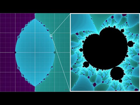
Piere Fatou and Gaston Julia built up a rich theory of what happens when rational functions are iterated in the years following World War 1, despite not having computers to visualize their results. One of the most popular examples is z^2 + c, where c is a constant. Starting with z=0, if c is changed, the second value will move in lockstep. If the value of c is such that the process remains bounded, it will be coloured black. If it is divergent, it will be coloured according to how quickly it rushes off to infinity, forming the iconic Mandelbrot set. This set is different from Newton’s fractal in that it is a parameter space, with a consistent seed value (z=0) and the parameter c changing the function itself. Alternatively, Newton’s fractal has a single unchanging function, with the pixels representing different seed values. The derivative of a complex function at a point is just the tangent line at that point, and so the derivative of z^2 is just a line with slope 2.And this is the same as saying that the function is increasing twice as fast as it moves away from the origin.
Whereas each pixel of the Mandelbrot set corresponds to a unique function, the images on the right each just correspond to a single function. As we change the parameter c, it changes the entire image on the right. The rule being applied is to color pixels black if the process remains bounded and then apply some kind of gradient to the ones that diverge away to infinity based on how quickly they diverge to infinity. In principle, there is some four-dimensional space of all combinations of c and z_0, and what we’re doing here is looking through individual two-dimensional slices of that pattern. The images on the right are often referred to as “Julia sets” or “Julia fractals”.
To set the stage for a more specific definition, a good place to start is to ask if there are any parts of the system that have some simple behavior, preferably the simplest possible behavior. In our example, that might mean asking when does the process just stay fixed in place, meaning f(z) = z. We call a value with this property a “fixed point” of the function. In the case of the functions arising from Newton’s method, by design they have a fixed point at the roots of the relevant polynomial.
More generally, any rational function will always have fixed points, since asking when this expression equals z can always be rearranged as finding the roots of some polynomial expression, and from the fundamental theorem of algebra this must have solutions, typically as many solutions as the highest degree in this expression.
Just asking about fixed points is maybe easy, but a key idea for understanding the full dynamics, and hence the diagrams that we’re looking at, is to understand stability. We say that a fixed point is attracting if nearby points tend to get drawn in towards it, and repelling if they’re pushed away. And this is something that you can actually compute explicitly using the derivative of the function. Symbolically, when you take derivatives of complex functions, it looks exactly the same as it would for real functions. Geometrically, the derivative of a complex function at a point is just the tangent line at that point, and so the derivative of z^2 is just a line with slope 2. This is the same as saying that the function is increasing twice as fast as it moves away from the origin. For example, at the input 1 the derivative of this particular function evaluates to be 2, and what that’s telling us is that if you look at a very small neighborhood around that input and you follow what happens to all the points in that little neighborhood as you apply the function, in this case $z^2$, then it looks just like you’re multiplying by 2. This is what a derivative of 2 means.
To take another example let’s look at the input $i$. We know that this function moves that input to the value -1, that’s $i^2$. But the added information that its derivative at this value is 2 times $i$ gives us the added picture that when you zoom in around that point and you look at the action of the function on this tiny neighborhood, it looks like multiplication by $2i$, which in this case is saying it looks like a 90 degree rotation combined with a expansion by a factor of 2. For the purposes of analyzing stability, the only thing we care about here is the growing and shrinking factor, the rotational part doesn’t matter. So if you compute the derivative of a function at its fixed point, and the absolute value of this result is less than one, it tells you that the fixed point is attracting, that nearby points tend to come in towards it. If that derivative has an absolute value bigger than one, it tells you the fixed point is repelling, it pushes away its neighbors.
For example if you work out the derivative of our Newton’s map expression, and you simplify a couple things a little bit, here’s what you would get out. So if $z$ is a fixed point, which in this context means that it’s one of the roots of the polynomial $p$, this derivative is not only smaller than one, it’s equal to zero. These are sometimes called “superattracting” fixed points, since it means that a neighborhood around these points doesn’t merely shrink, it shrinks a lot. And again this is kind of by design, since the intent of Newton’s method is to produce iterations that fall towards a root as quickly as they can.
Pulling up our $z^2 + c$ example, if you did the first exercise to find its fixed points, the next step would be to ask when is at least one of those fixed points is attracting. For what values of $c$ is this going to be true? And then if that’s not enough of a challenge, try using the result that you find to show that this condition corresponds to the main cardioid shape of the Mandelbrot set. This is something you can compute explicitly, it’s pretty cool.
A natural next step would be to ask about cycles, and this is where things really start to get interesting. If $f(z)$ is not $z$, but some other value, and then that value comes back to $z$, it means that you’ve fallen into a two-cycle. You could explicitly find these kinds of two-cycles by evaluating $f(f(z))$, and then setting it equal to $z$. For example with the $z^2 + c$ map, $f(f(z))$ expands out to look like this. It’s a little messy, but you know it’s not too terrible. The main thing to highlight is that it boils down to solving some degree four equation. You should note though that the fixed points will also be solutions to this equation, so technically the two-cycles are the solutions to this minus the solutions to the original fixed point equation.
And likewise you can use the same idea to look for n-cycles by composing $f$ with itself n different times. The explicit expressions that you would get quickly become insanely messy, but it’s still elucidating to ask how many cycles would you expect based on this hypothetical process.
If we stick with our simple $z^2 + c$ example, as you compose it with itself you get a polynomial with degree 4, and then one with degree 8, and then degree 16, and so on and so on exponentially growing the order of the polynomial. If you were to ask how many cycles there are with a period of one million, then the answer would be that it is equivalent to solving a polynomial expression of degree 2 to the one million. According to the Fundamental Theorem of Algebra, this would result in 2 to the one million points in the complex plane that cycle in this way. Additionally, for any rational map, there will always be values whose behavior falls into a cycle with period n. This ultimately boils down to solving a (likely insane) polynomial expression, and the number of periodic points will grow exponentially with n.
When it comes to Newton’s Map process, there is a non-zero chance that an initial guess can get trapped in an attracting cycle and never find a root. For example, if you were to find the roots of z^3 - 2z + 2, then if you start with a small cluster around the value zero, it will tend to get pulled in towards the cycle between 0 and 1.
It is also possible to visualize which cubic polynomials have attracting cycles. If the seed value never gets close enough to a root, then the pixel will be colored black. It is rare to see black pixels, but it can be done by tweaking the roots. Furthermore, there is a simple way to test whether or not a polynomial has an attracting cycle: look at the seed value which sits at the average of the three roots. If there is an attracting cycle, then this seed value will fall into it. It’s this property that gives rise to the fractal-like shapes.In other words, if there are any black points, this will be one of them. If you want to know where this magical fact comes from, it stems from a theorem of our good friend Fatou. He showed that if one of these rational maps has an attracting cycle, you can look at the values where the derivative of your iterated function equals zero, and at least one of those values has to fall into the cycle. That might seem like a little bit of a weird fact, but the loose intuition is that if a cycle is going to be attracting, at least one of its values should have a very small derivative, that’s where the shrinking will come from. And this in turn means that that value in the cycle sits near some point where the derivative is not merely small, but equal to zero. And that point ends up being close enough to get sucked into the cycle.
This fact also justifies why with the Mandelbrot set, where we’re only using one seed value z=0, it’s still enough to get us a very full and interesting picture. If there’s a stable cycle to be found, that one seed value is definitely going to find it. I feel like maybe I’m assigning a little too much homework and exercises today, but if you’re into that, yet another pleasing one would be to look back at the derivative expression that we found with our function that arises from Newton’s method and use this wonderful theorem of Fatou’s to show our magical fact about cubic polynomials, that it suffices to just check this midpoint over the roots. Honestly, though, all of those are details that you don’t really have to worry about. The upshot is that we can perform a test for whether or not one of these polynomials has an attracting cycle by looking at just a single point, not all of them. And because of this, we can actually generate a really cool diagram. And this is true more generally for any rational map: if you were to assign colors to regions based on which limiting behavior points fall into, like which limit point or which limit cycle or does it tend to infinity, then tiny circles that you draw either contain points with just one of those limiting behaviors, or they contain points with all of them. It’s never anything in between. So, in the case where there’s at least three colors, this property implies that our boundary could never be smooth since along a smooth segment you can draw a small enough circle that touches just two colors, not all of them. And empirically this is what we see. No matter how far you zoom in, these boundaries are always rough, and furthermore you might notice that as we zoom in you can always see all available colors within the frame. This doesn’t explain rough boundaries in the context where there’s only two limiting behaviors, but still it’s a loose end that I left in that video worth tying up, and it’s a nice excuse to bring in two important bits of terminology: Julia sets and Fatou sets.
If a point eventually falls into some stable predictable pattern, we say that it’s part of the Fatou set of our iterated function. And for all the maps that we’ve seen, this includes almost everything. The Julia set is everything else, which in the pictures we’ve seen would be the rough boundaries between the colored regions, what happens as you transition from one stable attractor to another. For example, the Julia set will include all of the repelling cycles and the repelling fixed points. A typical point from the Julia set, though, will not be a cycle, it’ll bounce around forever with no clear pattern.
If you look at a point in the Fatou set and you draw a small enough disk around it, as you follow the process that small disk will eventually shrink as you fall into whatever the relevant stable behavior is. Unless you’re going to infinity, but you could kind of think of that as the disc shrinking around infinity, but maybe that just confuses matters… By contrast, if you draw a small disc around a point on the Julia set, it tends to expand over time as the points from within that circle go off and kind of do their own things. In other words, points of the Julia set tend to behave chaotically. Their nearby neighbors, even very nearby, will eventually fall into qualitatively different behaviors.
But it’s not merely that this disk expands, a pretty surprising result, key to the multi-color property mentioned before, is that if you let this process play out that little disk eventually expands so much that it hits every single point on the complex plane, with at most two exceptions. This is known as the “stuff goes everywhere principle” of Julia sets. Okay, it’s not actually called that, in the source I was reading from it’s mentioned as a corollary to something known as Montel’s theorem, but it should be called that. In some sense what this is telling us is that the points of the Julia set are not merely chaotic, they’re kind of as chaotic as they possibly can be.
Here let me show you a little simulation using the newton’s map with a cluster of a few thousand points all starting from within a tiny tiny distance one one millionth from a point on the Julia set. Of course the stuff goes everywhere principle is about the uncountably infinitely many points that would lie within that distance, and that they eventually expand out to hit everything on the plane, except possibly two points, but this little cluster should still give the general idea. A small finite sample from that tiny disk gets sprayed all over the place in seemingly all directions. What this means for our purposes is that if there’s an attractive behavior of our map, like an attracting fixed point or an attracting cycle, you can be guaranteed that the values from that tiny disk around the point on the Julia set, no matter how small, will eventually fall into that attracting behavior. Even if there are three or more attracting behaviors, this gives us an explanation for why the Julia set is not smooth and why it has to be complicated.
This might not be entirely satisfying as it kicks the can one step down the road, raising the question of why this “stuff goes everywhere principle” is true in the first place. This comes from something called Montel’s theorem, which is a lot to cover, so I’m choosing not to go into the details. The proof I could find ends up leaning on something known as the j-function, which is a whole intricate story in its own right. I will of course leave links and resources in the description for anyone who is hungry to learn more. If you know of a simpler way to see why this principle is true, I’m definitely all ears.
I should also say, as a brief side note, that even though the pictures we’ve seen so far have a Julia set with an area of zero, it’s kind of the boundary between these regions. There are examples where the Julia set is the entire plane, and everything behaves chaotically, which is kind of wild.
The main takeaway for this particular section is the link between the chaos and the fractal. At first it seems like these are merely analogous to each other, but when you quantify just how chaotic some of the points are, that quantification leads us to an actual explanation for the rough fractal shape via this boundary property. Quite often you see chaos and fractals sort of married together in math, and it’s satisfying whenever that marriage comes with a logical link to it rather than two phenomena that just happened to coincide.