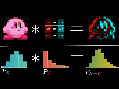
Suppose I give you two different lists of numbers or two different functions and I ask you to think of all the ways you might combine them to get a new list of numbers or a new function. One simple way to combine them is to add or multiply them term by term. Another way to combine them is through convolution. Convolution is a core construct in the theory of probability and is used a lot in solving differential equations, and is also used when multiplying two polynomials together. In this video, we will focus on the discrete case and build up to a clever algorithm for computing these. We will also discuss the continuous case in a second part. We will start with an example from probability - rolling a pair of dice and figuring out the chances of seeing various different sums. We can count up how many pairs have a given sum by arranging them in a grid and counting how many exist on each diagonal. Another way to visualize the same question is to picture the two sets of possibilities each in a row, but flipping around the second row. This way, all of the pairs that add up to seven line up vertically, and when the bottom row is slid to the right, the unique pair that adds up to two is the only one that aligns. That’s 18.And if you look at this output, you’ll see it looks like the list 4, 13, 28, 27, 18.
The convolution of two sequences, A and B (denoted with *), is a new list where the Nth element is a sum of all pairs of indices, I and J, such that the sum of those indices is equal to N. For example, the convolution of the list [1, 2, 3] and [4, 5, 6] is [4, 13, 28, 27, 18]. If you’d like, you can pull up your favorite programming language and library that includes various numerical operations and confirm that I’m not lying to you. For example, if you take the convolution of 1, 2, 3 against 4, 5, 6, you’ll get the result shown. We’ve seen one case where this is a natural and desirable operation, such as adding up to probability distributions. Another common example is a moving average. Imagine you have some long list of numbers and you take another smaller list of numbers that all add up to one. In this case, I just have a little list of five values and they’re all equal to one fifth. Then if we do this sliding window convolution process, each term in the convolution means multiplying each of the values from your data by one fifth and adding them all together, which is to say you’re taking an average of your data inside this little window. This gives you a smooth out version of the original data.
If we do a two dimensional analog of this, it gives us a fun algorithm for blurring a given image. At each iteration, we have a little 3x3 grid of values that marches along our original image, each one of which is one ninth. We multiply all these little values by the corresponding pixel that it sits on top of, and add them together, which gives us an average along each color channel and the corresponding pixel for the image on the right is defined to be that sum. The overall effect is that each one kind of bleeds into all of its neighbours, which gives us a blurrier version than the original.
If we modify this slightly, we can get a much more elegant blurring effect by choosing a different grid of values. In this case, I have a little 5x5 grid but the distinction is not so much its size. If we zoom in, we notice that the value in the middle is a lot bigger than the value towards the edges, which are all sampled from a bell curve known as a Gaussian distribution. That way, when we multiply all of these values by the corresponding pixel that they’re on top of, we’re giving a lot more weight to that central pixel and much less towards the ones out at the edge. As we saw before, the idea of a convolution is to take two arrays, one of which we call the kernel, and for every element in the first array, multiply the corresponding elements in the kernel and add them together. This gives a blurring effect which more authentically simulates the notion of putting your lens out of focus. However, blurring is far from the only thing that you can do with this idea. For instance, if the kernel is made up of positive and negative numbers (blue and red respectively), this will have the effect of detecting any variation in the pixel value as you move from left to right. This can be used to pick up on vertical edges in an image. Similarly, if the kernel is rotated so that it varies as you move from the top to the bottom, this will be picking up on all the horizontal edges.
Another thing to note is that in certain computer science contexts, the output of the convolution needs to be deliberately truncated to match the size of the original array. In addition, flipping the kernel before it marches across the original may feel strange, but it is an incredibly natural thing to do in the pure math context. Finally, there are faster algorithms to compute convolutions which can be useful for programming contexts. For example, if we have two polynomials each with N different coefficients and we know the outputs at N different points.Then that’s equivalent to having N equations and two unknowns, which can be solved for the two polynomials.
Each of the 100,000 random elements will be used to assess the run time of the convolve function from the Numpy library. On this computer, it averages at 4.87 seconds. However, if the FFT convolve function from the SciPy library is used instead, it only takes 4.3 milliseconds on average, resulting in a three orders of magnitude improvement.
The convolution process can be thought of as creating a multiplication table with all pairwise products and then adding up those pairwise products along the diagonals. This is especially natural when multiplying two polynomials, as it is equivalent to expanding out the full product and collecting like terms.
Multiplying two polynomials together is a point wise operation, which requires fewer operations than a convolution, which is O of N squared. If two polynomials are known at N distinct outputs, that’s enough to uniquely specify the polynomials and solve for them. And then, finally, compute the inverse fourier transform of that result.Which will give you the convolution of the two lists.
Imagine I tell you, I have some polynomial but I don’t tell you what the coefficients are, those are a mystery to you. In our example, you might think of this as the product that we’re trying to figure out. And then suppose I say, I’ll just tell you what the outputs of this polynomial would be if you inputted various different inputs like 0, 1, 2, 3 on and on. And I give you enough so that you have as many equations as you have unknowns. It even happens to be a linear system of equations so that’s nice. And in principle, at least, this should be enough to recover the coefficients.
So the rough algorithm outline then would be whenever you want to convolve two lists of numbers, you treat them like they’re coefficients of two polynomials. You sample those polynomials at enough outputs, multiply those samples point wise, and then solve the system to recover the coefficients as a sneaky backdoor way to find the convolution. And as I’ve stated it so far, at least, some of you could rightfully complain, Grant, that is an idiotic plan. Because for one thing, just calculating all these samples for one of the polynomials we know, already takes on the order of N squared operations. Not to mention, solving that system is certainly going to be computationally as difficult as just doing the convolution in the first place.
So like, sure, we have this connection between multiplication and convolutions but all of the complexity happens in translating from one viewpoint to the other. But there is a trick. And those of you who know about fourier transforms and the FFT algorithm, might see where this is going. If you’re unfamiliar with these topics, what I’m about to say might seem completely out of the blue. Just know that there are certain paths you could have walked in math that make this more of an expected step.
Basically the idea is that we have a freedom of choice here. If instead of evaluating as some arbitrary set of inputs like 0, 1, 2, 3 on and on, you choose to evaluate on a very specially selected set of complex numbers. Specifically the ones that sit evenly spaced on the unit circle, what are known as the roots of unity. This gives us a friendlier system. The basic idea is that by finding a number where taking its powers falls into this cycling pattern, it means that the system we generate is going to have a lot of redundancy in the different terms that you’re calculating. And by being clever about how you leverage that redundancy, you can save yourself a lot of work.
This set of outputs that I’ve written has a special name. It’s called the discrete fourier transform of the coefficients. And if you want to learn more, I actually did another lecture for that same Julia MIT class, all about discrete fourier transforms. And there’s also a really excellent video on the channel reducible, talking about the fast fourier transform, which is an algorithm for computing these more quickly. Also Veritasium recently did a really good video on FFTs so you’ve got lots of options.
And that fast algorithm really is the point for us. Again, because of all this redundancy, there exist a method to go from the coefficients to all of these outputs. Where instead of doing on the order of N squared operations, you do on the order of N times the log of N operations which is much much better as you scale to big lists. And importantly, this FFT algorithm goes both ways. It also lets you go from the outputs to the coefficients.
Though bringing it all together, let’s look back at our algorithm outline. Now, we can say, whenever you’re given two long lists of numbers and you want to take their convolution, first, compute the fast fourier transform of each one of them. Which in the back of your mind, you can just think of as treating them like they’re the coefficients of a polynomial and evaluating it at a very specially selected set of points. Then, multiply together the two results that you just got, point wise, which is nice and fast. And then, finally, compute the inverse fourier transform of that result. Which will give you the convolution of the two lists. Multiplying two numbers is essentially a convolution between the digits of those numbers, and with the existence of a fast algorithm, it’s possible to find their product faster than the method we learn in elementary school. This fast algorithm only requires O of N log N operations, which is much faster than the O of N squared operations required in the elementary school method. This is especially useful in contexts where convolutions show up, such as multiplying two polynomials, adding probability distributions to large image processing, and more. It’s a great example of why it’s exciting to see math concepts show up in a variety of seemingly unrelated areas. Next, we will turn our attention to the continuous case with a special focus on probability distributions.