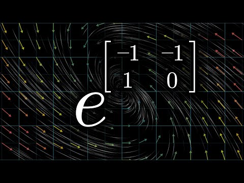
Let me pull out an old differential equations textbook I learned from in college, and let’s turn to this funny little exercise in here that asks the reader to compute $e^A$, where $A$, we’re told, is going to be a matrix, and the insinuation seems to be that the result will also be a matrix. It then offers several examples for what you might plug in for $A$. Now, taken out of context, putting a matrix in an exponent like this probably seems like total nonsense, but what it refers to is an extremely beautiful operation, and the reason it shows up in this book is that it’s useful, it’s used to solve a very important class of differential equations. In turn, given that the universe is often written in the language of differential equations, you see it pop up in physics all the time too, especially in quantum mechanics, where matrix exponents are littered throughout the place, they play a particularly prominent role. This has a lot to do with Shrödinger’s equation, which we’ll touch on a bit later. And it also may help in understanding your romantic relationships, but again, all in due time.
A big part of the reason I want to cover this topic is that there’s an extremely nice way to visualize what matrix exponents are actually doing using flow, that not a lot of people seem to talk about. But for the bulk of this chapter, let’s start by laying out what exactly the operation actually is, and then see if we can get a feel for what kinds of problems it helps us to solve.
The first thing you should know is that this is not some bizarre way to multiply the constant $e$ by itself multiple times; you would be right to call that nonsense. The actual definition is related to a certain infinite polynomial describing for real number powers of $e$, what we call its Taylor series. For example, if I took the number 2 and plugged it into this polynomial, then as you add more and more terms, each of which looks like some power of 2 divided by some factorial…the sum approaches a number near 7.389, and this number is precisely $e^2$. If you increment this input by 1, then somewhat miraculously no matter where you started from the effect on the output is always to multiply it by another factor of $e$.
For reasons that you’re going to see a bit, mathematicians became interested in plugging all kinds of things into this polynomial, things like complex numbers, and for our purposes today, matrices, even when those objects do not immediately make sense as exponents. What some authors do is give this infinite polynomial the name “exp” when you plug in more exotic inputs. It’s a gentle nod to the connection that this has to exponential functions in the case of real numbers, even though obviously these inputs don’t make sense as exponents. However, an equally common convention is to give a much less gentle nod to the connection and just abbreviate the whole thing as $e^A$, whether that’s a complex number, or a matrix, or all sorts of more exotic objects.
So while this equation is a theorem for real numbers, it’s a definition for more exotic inputs. Cynically, you could call this a blatant abuse of notation. More charitably, you might view it as an example of the beautiful cycle between discovery and invention in math. In either case, plugging in a matrix, even to a polynomial, might seem a little strange, so let’s be clear on what we mean here. The matrix needs to have the same number of rows and columns. That way you can multiply it by itself according to the usual rules of matrix multiplication. This is what we mean by squaring it. Similarly, if you were to take that result, and then multiply it by the original matrix again, this is what we mean by cubing the matrix. If you carry on like this, you can take any whole power of a matrix, it’s perfectly sensible. So if she’s expressing cool disinterest, he starts to lose interest, and vice versa.
In this context, powers still mean exactly what you’d expect, repeated multiplication. Each term of this polynomial is scaled by 1/n!, and with matrices, this means that you multiply each component by that number. Likewise, it always makes sense to add two matrices, this is something you do term-by-term. The astute among you might ask how sensible it is to take this out to infinity, which would be a great question, one that I’m largely going to postpone the answer to, but I can show you one pretty fun example here now.
Take this 2x2 matrix that has -π and π sitting off its diagonal entries. Let’s see what the sum gives. The first term is the identity matrix, this is actually what we mean by definition when we raise a matrix to the 0th power. Then we add in the matrix itself, which gives us the pi-off-the-diagonal terms. And then add half of the matrix squared, and continuing on I’ll have the computer keep adding more and more terms, each of which requires taking one more matrix product to get a new power and adding it to a running tally. And as it keeps going, it seems to be approaching a stable value, which is around -1 times the identity matrix. In this sense, we say the sum equals that negative identity.
By the end of this video, my hope is that this particular fact comes to make total sense to you, for any of you familiar with Euler’s famous identity, this is essentially the matrix version of that. It turns out that in general, no matter what matrix you start with, as you add more and more terms you eventually approach some stable value. Though sometimes it can take quite a while before you get there.
Just seeing the definition like this, in isolation, raises all kinds of questions. Most notably, why would mathematicians and physicists be interested in torturing their poor matrices this way, what problems are they trying to solve? And if you’re anything like me, a new operation is only satisfying when you have a clear view of what it’s trying to do, some sense of how to predict the output based on the input before you actually crunch the numbers. How on earth could you have predicted that the matrix with pi off the diagonals results in the negative identity matrix like this?
Often in math, you should view the definition not as a starting point, but as a target. Contrary to the structure of textbooks, mathematicians do not start by making definitions, and then listing a lot of theorems and proving them, and then showing some examples. The process of discovering math typically goes the other way around. They start by chewing on specific problems and then generalizing those problems, then coming up with constructs that might be helpful in those general cases. And only then do you write down a new definition, or extend an old one.
As to what sorts of specific examples might motivate matrix exponents, two come to mind, one involving relationships, and other quantum mechanics. Let’s start with relationships. Suppose we have two lovers, let’s call them Romeo and Juliet. And let’s let x represent Juliet’s love for Romeo, and y represent his love for her, both of which are going to be values that change with time. This is an example that we actually touched on in chapter 1, it’s based on a Steven Strogatz article, but it’s okay if you didn’t see that.
The way their relationship works is that the rate at which Juliet’s love for Romeo changes, the derivative of this value, is equal to the -1 times Romeo’s love for her. So in other words, when Romeo is expressing cool disinterest, that’ when Juliet’s feelings actually increase, whereas if he becomes too infatuated, her interest will start to fade. Romeo, on the other hand, is the opposite, the rate of change of his love is equal to Juliet’s love. So if she’s expressing cool disinterest, he starts to lose interest, and vice versa. Romeo and Juliet’s relationship can be pictured as a point in a 2-dimensional space, with Juliet’s feelings represented by the x-coordinate and Romeo’s by the y-coordinate. This point is subject to a system of differential equations: if Juliet loves him, his feelings grow, whereas if she is mad at him, his affections tend to decrease. This is represented by a 90-degree rotation matrix, which takes the first basis vector to [0, 1] and the second to [-1, 0]. To solve this equation, one can use matrix exponents or a simpler geometric approach. What our equation is saying is that the rate of change of Romeo and Juliet’s position in this state space is like a 90-degree rotation of their position vector. This rotation about the origin results in a velocity of constant length, as the rate of change has no component in the direction of position. This means that for each unit of time, the distance covered is equal to one radius of arc length along the circle. This can be expressed with a more general rotation matrix, which takes the first basis vector to [cos(t), sin(t)] and the second basis vector to [-sin(t), cos(t)]. To solve the system, we can multiply this matrix by the initial state to predict where Romeo and Juliet will end up after a certain amount of time.
The same concept applies to Shrödinger’s equation, which is the fundamental equation describing how systems in quantum mechanics change over time. This equation refers to a certain vector which packages together all the information about the system, and the rate of change of this vector is proportional to the vector itself. This is a highly important equation, and is much simpler to visualize in one-dimensional cases, where the higher the value of the graph, the steeper its slope. Calculus students all learn about how the derivative of $e^{rt}$ is $r$ times itself. In other words, this self-reinforcing growth is the same thing as exponential growth, and $e^{rt}$ solves this equation. Actually, a better way to think about it is that there are many different solutions to this equation, one for each initial condition, something like an initial investment size or initial population, which we’ll just call $x_0$. Notice, by the way, how the higher the value for $x_0$, the higher the initial slope of the resulting solution, which should make complete sense given the equation. The function $e^{rt}$ is just a solution when the initial condition is 1. But! If you multiply by any other initial condition, you get a new function that still satisfies the property, it still has a derivative which is $r$ times itself. But this time it starts at $x_0$, since $e^0$ is 1. This is worth highlighting before we generalize to more dimensions: Do not think of the exponential part as a solution in and of itself. Think of it as something which acts on an initial condition in order to give a solution.
You see, up in the 2-dimensional case, when we have a changing vector whose rate of change is constrained to be some matrix times itself, what the solution looks like is also an exponential term acting on a given initial condition. But the exponential part, in that case, will produce a matrix that changes with time, and the initial condition is a vector. In fact, you should think of the definition of matrix exponentiation as being heavily motivated by making sure this is true.
For example, if we look back at the system that popped up with Romeo and Juliet, the claim now is that solutions look like $e$ raised to this [[0, -1], [1, 0]] matrix all times time, multiplied by some initial condition. But we’ve already seen the solution in this case, we know it looks like a rotation matrix times the initial condition. So let’s take a moment to roll up our sleeves and compute the exponential term using the definition I mentioned at the start, and see if it lines up.
Remember, writing $e$ to the power of a matrix is a shorthand, a shorthand for plugging it into this long infinite polynomial, the Taylor series of $e^x$. I know it might seem pretty complicated to do this, but trust me, it’s very satisfying how this particular one turns out. If you actually sit down and you compute successive powers of this matrix, what you’d notice is that they fall into a cycling pattern every four iterations. This should make sense, given that we know it’s a 90-degree rotation matrix. So when you add together all infinitely many matrices term-by-term, each term in the result looks like a polynomial in $t$ with some nice cycling pattern in the coefficients, all of them scaled by the relevant factorial term. Those of you who are savvy with Taylor series might be able to recognize that each one of these components is the Taylor series for either sine or cosine, though in that top right corner’s case it’s actually $-\sin(t)$. So what we get from the computation is exactly the rotation matrix we had from before!
To me, this is extremely beautiful. We have two completely different ways of reasoning about the same system and they give us the same answer. I mean it’s reassuring that they do, but it is wild just how different the mode of thought is when you’re chugging through the polynomial vs. when you’re geometrically reasoning about what a velocity perpendicular to a position must imply. Hopefully the fact that these line up inspires a little confidence in the claim that matrix exponents really do solve systems like this. This explains the computation we saw at the start, with the matrix that had -π and π off the diagonal, producing the negative identity. This expression is exponentiating a 90-degree rotation matrix times π, which is another way to describe what the Romeo-Juliet setup does after π units of time. As we now know, that has the effect of rotating everything by 180-degrees in this state space, which is the same as multiplying everything by -1. Also, for any of you familiar with imaginary number exponents, this example is probably ringing a ton of bells. It is 100% analogous. In fact, we could have framed the entire example where Romeo and Juliet’s feelings were packaged into a complex number, and the rate of change of that complex number would have been i times itself since multiplication by i also acts like a 90-degree rotation. The same exact line of reasoning, both analytic and geometric, would have led to this whole idea that e^(it) describes rotations.
There are actually two of many different examples throughout math and physics when you find yourself exponentiating some object which acts as a 90-degree rotation, times time. It shows up with quaternions or many of the matrices that pop up in quantum mechanics. In all of these cases, we have this really neat general idea that if you take some operation that rotates 90-degrees in some plane, often it’s a plane in some high-dimensional space we can’t visualize, then what we get by exponentiation that operation times time is something that generates all other rotations in that same plane. One of the more complicated variations on this same theme is Shrödinger’s equation. It’s not just that it has the derivative-of-a-state-equals-some-matrix-times-that-state form. The nature of the relevant matrix here is such that this equation also describes a kind of rotation, though in many applications of Schrödinger’s equation it will be a rotation inside a kind of function space. It’s a little more involved, though, because typically there’s a combination of many different rotations.
It takes time to really dig into this equation, and I’d love to do that in a later chapter. But right now I cannot help but at least allude to the fact that this imaginary unit i that sits so impishly in such a fundamental equation for all of the universe, is playing basically the same role as the matrix from our Romeo-Juilet example. What this i communicates is that the rate of change of a certain state is, in a sense, perpendicular to that state, and hence that the way things have to evolve over time will involve a kind of oscillation.
But matrix exponentiation can do so much more than just rotation. You can always visualize these sorts of differential equations using a vector field. The idea is that this equation tells us that the velocity of a state is entirely determined by its position. So what we do is go to every point in this space, and draw a little vector indicating what the velocity of a state must be if it passes through that point. For our type of equation, this means that we go to each point v in space, and we attach the vector M times v. To intuitively understand how any given initial condition will evolve, you let it flow along this field, with a velocity always matching whatever vector it’s sitting on at any given point in time. So if the claim is that solutions to this equation look like e^(Mt) times some initial condition, it means you can visualize what the matrix e^(Mt) does by letting every possible initial condition flow along this field for t units of time. The transition from start to finish is described by whatever matrix pops out from the computation for e^(Mt). In our main example with the 90-degree rotation matrix, the vector field looks like this, and as we saw e^(Mt) describes rotation in that case, which lines up with flow along this field. As another example, the Shakespearian classic Romeo and Juliet might have equations that look a little different. Juliet’s rule is symmetric with Romeo’s, and both of them are inclined to get carried away in response to each other’s feelings. The vector field is defined by going to each point v in space and attaching the vector M times v. This means that the rate of change of a state must always equal M times itself. If Romeo and Juliet start in the upper-right half of the plane, their feelings will feed off of each other and they both tend towards infinity. However, if they’re in the other half of the plane, they will stay true to their Capulet and Montague family traditions.
Before calculating the exponential of this particular matrix, one can have an intuitive sense of what the answer should look like. The resulting matrix should describe the transition from time 0 to time t, which, if you look at the field, seems to indicate that it will squish along one diagonal while stretching along another, getting more extreme as t gets larger. To verify this, one must write out the full polynomial that defines e^(Mt) and multiply by some initial condition vector on the right. Then, by taking the derivative of this with respect to t, one can factor out the expression and solve the equation.
In the next chapter, we will discuss the properties that this operation has, such as its relationship with eigenvectors and eigenvalues. We will also explore what it means to raise e to the power of the derivative operator.