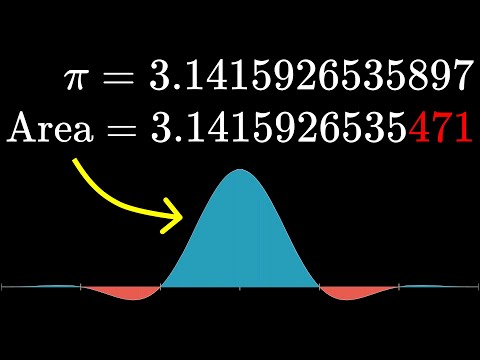
Sometimes it feels like the universe is just messing with you. I have up on screen here a sequence of computations and don’t worry, in a moment we’re going to unpack and visualize what each one is really saying. What I want you to notice is how the sequence follows a very predictable, if random seeming pattern, and how each computation happens to equal pi. And if you are just messing around evaluating these on a computer for some reason, you might think that this was a pattern that would go on forever. But it doesn’t. At some point, it stops and instead of equaling pi, you get a value which is just barely, barely less than pi. Alright, let’s dig into what’s going on here. The main character in the story today is the function sin of X divided by X. This actually comes up commonly enough in math and engineering that it gets its own name, “sinc” and the way you might think about it is by starting with a normal oscillating sin curve and then sort of squishing it down as you get far away from zero by multiplying it by 1 over X and the astute among you might ask about what happens at X equals 0 since when you plug that in, it looks like dividing zero by zero and then the even more astute among you may fresh out of a calculus class could point out that for values closer and closer to zero, the function gets closer and closer to one. So, if we simply redefine the sinc function at 0 to equal 1, you get a nice continuous curve. All of that is a little by the by because the thing we actually care about is the integral of this curve from negative infinity to infinity. Which you think of as meaning the area between the curve and the X axis, or more precisely the signed area. Meaning you add all the area bound by the positive parts of the graph in the X axis and you subtract all of the parts found by the negative parts of the graph and the X axis. Like we saw at the start, it happens to be the case that this evaluates to be exactly pi, which is nice and also a little weird and it’s not entirely clear how you would approach this with the usual tools of calculus. Towards the end of the video, I’ll share the trick for how you would do this.
Progressing on with the sequence I opened with, the next step is to take a copy of the sinc function where you plug in X/3, which will basically look like the same graph but stretched out horizontal by a factor of three. When we multiply these two functions together, we get a much more complicated wave whose mass seems to be more concentrated towards the middle and with any usual functions, you would expect this completely changes the area. You can’t just randomly modify an integral like this and expect nothing to change. So already, it’s a little bit weird that this result also equals pi, that nothing has changed. That’s another mystery you should add to your list. And the next step in the sequence was to take an even more stretched out version of this sinc function by a factor of 5, multiply that by what we already have and again, look at the signed area underneath the whole curve, which again equals pi. And it continues on like this; with each iteration, we stretch out by a new odd number and multiply that into what we have. One thing you might notice is how except that the input X equals 0, every single part of this function is progressively getting multiplied by something that’s smaller than one. So you would expect as the sequence progresses for things to get squished down more and more and if anything, you would expect the area to be getting smaller. Eventually, that is exactly what happens but what’s bizarre is that it stays so stable for so long and of course, more pertinently, that when it does break at the value 15 it does so by the tiniest tiny amount. So, the value of the second iteration at zero is one.Now, the third iteration is going to be the same kind of moving average but now with a window that’s one fourth wide.So, the distance between the edges of the plateaus is one minus one fourth and then the value of the third iteration at zero is going to be one minus one fourth.For the fourth iteration, the window is one fifth wide, so the distance between the plateaus is one minus one fifth and the value of the fourth iteration at zero is going to be one minus one fifth.
The Borwein father-son pair described a phenomenon in a paper, where they found that a certain fraction of pi with a numerator and denominator of around 400 billion billion billion was the exact value of an integral. This was initially assumed to be a numerical error, but it was in fact a real phenomenon. Furthermore, when including another factor 2cos(x) into the integrals, the pattern was found to stay equal to pi for much longer, until it broke at the number 113, and even then the break was only by a very subtle amount.
The natural question then arises - what is going on here? A seemingly unrelated phenomenon was found to show a similar pattern, where a function called rect(x) was defined to equal 1 if the input was between -1/2 and 1/2, and 0 otherwise. This was the first in a sequence of functions, and each new function was a kind of moving average of the previous one. The value of the function at the input zero stayed stable for a while before it broke at the number 15, by just a tiny amount. It was then discovered that this phenomenon was secretly the same as all the integral expressions but in disguise. For the next iteration, we’re going to take a moving average of the last function, but this time with a window width of 1/5th. This will result in a smoother version of the previous function, with the value of the bottom function equalling one when the window is entirely inside the plateau of the previous function. The length of this plateau will be 1-1/3 minus the window width, 1/5th.
When we do one more iteration with 1/7th, the plateau gets smaller by the same amount, and with 1/9, the plateau gets smaller again. As we keep going, the plateau gets thinner and thinner, and just outside of the plateau, the function is very close to one.
The point at which this breaks is when we slide a window with width 1/15th across the whole thing - the previous plateau is then thinner than the window itself, and the output of the function at the input of zero is ever so slightly smaller than one. This is analogous to the integrals we saw earlier, where the pattern initially looks stable (i.e. pi, pi, pi, pi, pi) until it falls short just barely.
The same setup with a function that has an even longer plateau (stretching from x = -1 to 1) will take a lot longer for the windows to eat into the whole plateau. Specifically, it takes until the number 113 is reached for the sum of the reciprocals of the odd numbers to be bigger than two. This corresponds to the fact that the integral pattern continues until 113 is reached. There is nothing special about the reciprocals of odd numbers - one third, one fifth, one seventh - highlighted by the Borweins in their paper that made the sequence mildly famous in nerd circles. More generally, we could be inserting any sequence of positive numbers into those sinc functions and as long as the sum of those numbers is less than one, our expression will equal pi. However, as soon as they become bigger than one, our expression drops a little below pi. The connection between these two situations comes down to the fact that the sinc function (with the pi on the inside) is related to the rect function using a Fourier Transform. This is a nice thing about Fourier Transforms for functions that are symmetric about the Y axis, that is its own inverse. The slightly more general fact that we need to show is how when you transform the stretched out version of our sinc function where you stretch it horizontally by a factor of K, what you get is a stretched and squished version of this rect function. But of course, all of these are just meaningless words and terminology unless you can actually do something upon making this translation. And the real idea behind why Fourier Transforms are such a useful thing for math is that when you take statements and questions about a particular function and then you look at what they correspond to with respect to the transformed version of that function, those statements and questions often look very very different in this new language, and sometimes it makes the questions a lot easier to answer.
For example, one very nice little fact, another thing on our list of things to show, is that if you want to compute the integral of some function from negative infinity to infinity, this signed area under the entirety of its curve, it’s the same thing as simply evaluating the Fourier Transformed version of that function at the input zero. This is a fact that will actually just pop right out of the definition and representative of a more general vibe that every individual output of the Fourier Transform function on the right corresponds to some kind of global information about the original function on the left.
In our specific case, it means if you believe me that this sinc function and the rect function are related with the Fourier Transform like this, it explains the integral which is otherwise a very tricky thing to compute because it’s saying all that signed area is the same thing as evaluating rect at zero which is just one.
Now, you could complain - surely this just moves the bump under the rug. Surely computing this Fourier Transform, whatever that looks like would be as hard as computing the original integral. But the idea is that there’s lots of tips and tricks for computing these Fourier Transforms and moreover that when you do, it tells you a lot more information than just that integral. You get a lot of bang for your buck out of doing the computation.
Now, the other key fact that will explain the connection we’re hunting for is that if you have two different functions and you take their product and then you take the Fourier Transform of that product, it would be the same thing as if you individually took the Fourier Transforms of your original function and then combined them using a new kind of operation that we’ll talk all about in the next video known as a Convolution.
Now, even though there’s a lot to be explained with convolutions, the upshot will be that in our specific case with these rectangular functions, taking a convolution looks just like one of the moving averages that we’ve been talking about this whole time. Combined with our previous fact that integrating in one context looks like evaluating at zero in another context, if you believe me, that multiplying in one context corresponds to this new operation, convolutions, which for our example you should just think of as moving averages, that will explain why multiplying more and more of these sinc functions together can be thought about in terms of these progressive moving averages and always evaluating at zero, which in turn gives a really lovely intuition for why you would expect such a stable value before eventually something breaks down as the edges of the plateau inch closer and closer to the center.
This last key fact by the way has a special name, it’s called the Convolution Theorem and again, it’s something that we’ll go into much more deeply. I recognize that it’s maybe a little unsatisfying to end things here by laying down three magical facts and saying “everything follows from those”, but hopefully this gives you a little glimpse of why powerful tools like Fourier Transforms can be so useful for tricky problems. It’s a systematic way to provide a shift in perspective where hard problems can sometimes look easier. Hopefully, this has provided some motivation to learn about the convolution theorem - an incredibly useful tool. As an added bonus, the convolution theorem can be used to create an algorithm that can perform the product of two large numbers much more quickly than one would expect. With that, I’ll see you in the next video!