The basic function underlying a normal distribution, also known as a Gaussian, is e to the negative x squared. But you might wonder “Why this function?” Of all the expressions we could dream up that give you some symmetric smooth graph with mass concentrated towards the middle, why is it that the theory of probability seems to have a special place in its heart for this particular expression? For the last many videos, I’ve been hinting at an answer to this question and here we’ll finally arrive at something like a satisfying answer.
As a quick refresher on where we are - a couple videos ago, we talked about the Central Limit Theorem which describes how as you add multiple copies of a random variable, for example rolling a weighted die many different times or letting a ball bounce off of a peg repeatedly, then the distribution describing that sum tends to look approximately like a normal distribution. What the Central Limit Theorem says is as you make that sum bigger and bigger under appropriate conditions, that approximation to a normal becomes better and better. But I never explained why this is actually true, we only talked about what it’s claiming.
In the last video, we started talking about the math involved in adding two random variables. If you have two random variables each following some distribution, then to find the distribution describing the sum of those variables, you compute something known as a Convolution between the two original functions. And we spent a lot of time building up two distinct ways to visualize what this convolution operation really is.
Today, our basic job is to work through a example which is to ask what happens when you add two normally distributed random variables which, as you know by now, is the same as asking what do you get if you compute a convolution between two Gaussian functions. I’d like to share an especially pleasing visual way that you can think about this calculation which hopefully offers some sense of what makes the E to the negative X squared function special in the first place.
After we walk through it, we’ll talk about how this calculation is one of the steps involved in proving the Central Limit Theorem, it’s the step that answers the question of why a Gaussian and not something else is the central limit. But first, let’s dive in.
The full formula for a Gaussian is more complicated than just e to the negative x squared. The exponent is typically written as negative one-half times X divided by Sigma squared, where Sigma describes the spread of the distribution. Specifically the standard deviation. All of this needs to be multiplied by a fraction on the front which is there to make sure that the area under the curve is one making it a valid probability distribution. And if you want to consider distributions that aren’t necessarily centred at zero, you would also throw another parameter, µ into the exponent like this. Although for everything we’ll be doing here, we just consider centred distributions.
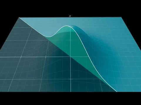
Now, if you look at our central goal for today, which is to compute a convolution between two Gaussian functions, the direct way to do this would be to take the definition of a convolution - this integral expression we built up the last video and then to plug in for each one of the functions involved the formula for a Gaussian. It’s kind of a lot of symbols when you throw it all together but more than anything working this out is an exercise in completing the square and there’s nothing wrong with that. That will get you the answer that you want but of course you know me, I’m a sucker for visual intuition and in this case, there’s another way to think about it that I haven’t seen written about before that offers a very nice connection to other aspects of this distribution like the presence of pi and certain ways to derive where it comes from. So, the way to compute the convolution of two copies of e to the negative x squared is to look at a slice over the line x + y = s and consider the area under that slice. Due to the rotational symmetry of the 3D graph, this area is equal to the area of a slice parallel to the y-axis, which is much easier to calculate. This area can be calculated by taking an integral with respect to y, with the value of x being equal to the constant s divided by the square root of two. The second step is to show that the shape that emerges is in fact a Gaussian.The point is that the result we just derived is the reason why this second step works.The convolution between two Gaussians is another Gaussian and that’s what makes the Central Limit Theorem so powerful.
The important point to note is that all of the stuff involving s is now entirely separate from the integrated variable. This remaining integral is a bit tricky; I did a whole video on it, which is actually quite famous. The point is that it’s just a number, which happens to be the square root of π, but what really matters is that it’s something with no dependence on s. This is our answer: the expression for the area of these slices as a function of s is e^{-s^2/2} scaled by some constant. This is a bell curve, another Gaussian just stretched out a bit due to the two in the exponent.
Technically, the convolution evaluated at s is not quite this area, but rather this area divided by the square root of two. This factor gets baked into the constant, so what really matters is the conclusion that a convolution between two Gaussians is itself another Gaussian. This result is very special, as almost always you end up with a completely different kind of function.
The Central Limit Theorem states that if you repeatedly add copies of a random variable to itself (mathematically, computing convolutions against a given distribution), then after appropriate shifting and rescaling, the tendency is always to approach a normal distribution. This computation that we just did is the reason that the function at the heart of the Central Limit Theorem is a Gaussian in the first place, and not some other function. It is also the reason why the second step of the proof of the theorem works. Going beyond what I want to discuss here, you often use objects called Moment-generating functions that suggest there must be some universal shape in a big family of distributions. Step two is proving that the convolution of two Gaussians gives another Gaussian, meaning it’s a fixed point and the only thing it can approach is itself. This implies that the Gaussian must be the universal shape. This calculation can be done directly with definitions, or with a geometric argument leveraging the rotational symmetry of the graph. This connects to the Herschel-Maxwell derivation of a Gaussian, the classic proof for why pi is in the formula, and an approach leveraging entropy, all of which can be explored further with the links in the description. If you want to stay up to date with new videos and other projects, there is a mailing list which I post sparingly to.