Why this particular one?
**You may have heard the phrase “The Unreasonable Effectiveness of Mathematics in the Natural Sciences.” This was the title of a paper by the physicist Eugene Wigner but even more fun than the title is the way that he chooses to open it. The paper begins quote, “There is a story about two friends who were classmates in high school…” talking about their jobs. One of them became a statistician and was working on population trends. They showed a reprint to their former classmates and the reprint started as usual with the Gaussian distribution. The statistician explained to the former classmate the meaning of the symbols for the actual population, the average population and so on. The classmate was incredulous and was not quite sure whether the statistician was pulling their leg. “How can you know that?” was the query and “What is this symbol over here?” “Oh”, said the statistician. “This is pi.” “What is that?” “The ratio of the circumference of a circle to its diameter.” “Well, now you’re pushing the joke too far.”, said the classmate. “Surely, the population has nothing to do with the circumference of a circle.” In the paper, Wigner then goes on to talk about the more general phenomenon of concepts in pure math seeming to find applications that extend strangely beyond what their definitions would suggest.
But I would like to stay focused on this particular anecdote and the question that the statistician’s friend is getting at. You see, there is a very beautiful and classic proof that explains the pi inside the formula for a normal distribution and despite there being a number of other really great explanations online, see some links in the description, I cannot help but indulge in the pleasure of reanimating it here. For one thing, there is a fun side note that I didn’t learn until recently about how you can use this proof to derive the volumes of higher dimensional spheres. But much more importantly than that, what I really want to do is try to go beyond the classic proof. Consider this hypothetical statistician’s friend. What I want to ask is, can we find an explanation that would satisfy their disbelief? You see, they’re not just asking for some pure math proof about a function that was handed down to them on high. The friend’s incredulity was that circles should have anything to do with population statistics. Until we fully draw that connecting line, we should consider the task incomplete.
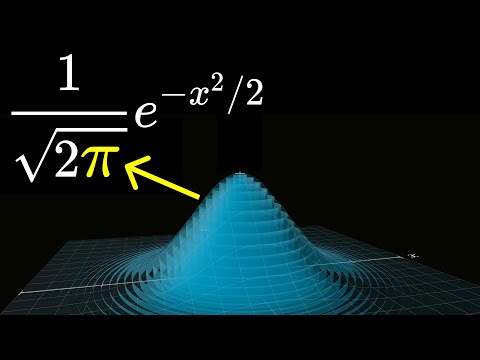
Those of you who watched the last video on the Central Limit Theorem will have some of the backdrop here because there we broke down the formula for a normal distribution, which is also called a Gaussian Distribution and when you strip away all of the different parameters and the constants, the basic function that describes the bell curve shape is e^-x^2. And the reason that pi showed up in the final formula was that the area underneath this curve works out, as you will see in a couple minutes, to be the square root of pi. So, what that meant for us was that at some point we needed to divide out by that square root of pi to make sure that the area under the curve is 1, which is a requirement before you can interpret it as a probability distribution.
In the full formula that you would see, say in a stats book, this gets mixed together with some of the other constants. But in its purest form, that pi originates from the area underneath this curve. So, step number one for you and me is to explain that area. But I want to emphasize it’s not the last step. To satisfy the question raised by that hypothetical statistician’s friend, we need to go further. We need to also answer why is it that this function e^-x^2 from is so special in the first place. I mean, there are lots of different formulas you could write down that would give a shape that you know, vaguely bulges in the middle and tapers out on either side. Why this particular one? So, let’s see what this does for us.
Why does this particular function hold such a special place in statistics? To answer this question, let’s explore the connection between the proof that explains why pi shows up and the Central Limit Theorem. As discussed in the last video, the Central Limit Theorem explains when a normal distribution can be expected to arise in nature.
To find the area underneath the curve, the tool used is an integral. To approximate the area, many rectangles are used, each with a height of the function above that point and a width of some small number. The sum of all the areas of these rectangles, for values of x ranging from negative infinity to infinity, is what the notation dx implies.
Calculus usually provides a way to answer this question, however, for this particular function it is not possible to find an antiderivative. Even though an antiderivative exists, it cannot be expressed using polynomial expressions, trigonometric functions, exponentials or any combination of these. To solve this problem, a new trick is needed.
The first step of this trick is to bump the problem up one dimension, so that instead of asking for the area under a bell curve, we ask for the volume underneath the bell surface. This higher dimensional function takes in two inputs, X and Y, and the distance of the point from the origin is labelled as “r”. The function is then e^-r^2. This gives the function a circular symmetry, and when graphed in three dimensions, it has a rotational symmetry about the Z axis. Math tends to reward when its symmetries are respected, so let’s see what this does for us. For a question of computing the volume underneath the surface, we can respect the symmetry and imagine integrating together a bunch of thin little cylinders underneath that surface. Making this more quantitative, let’s focus on just one of those cylindrical shells, where its area is going to be the circumference of that shell times the height. We can think of it as something like the label on a soup can that we can unwrap into a rectangle. The circumference of the cylinder, which is the top side of that rectangle is going to be 2$\pi$ times the radius and the height of our cylinder, the other side of our rectangle is the height of the surface at this point, which by definition is the value of our function associated with that radius, which like I said earlier, you can think of as $e^{-r^2}$.
Now the real way you want to think about this is to give that a little bit of thickness which we’ll call “$dr$” so that the volume that it represents is approximately that area we just looked at multiplied by this thickness, $dr$. Our task now is to integrate together or add together all of these different cylinders as our range is between zero and infinity. Or more precisely, we consider what happens as that thickness gets thinner and thinner approaching zero and we add together the volumes of the many many many different thin cylinders that sit underneath that curve.
We can factor the $\pi$ outside that integral and the stuff inside that integral, having picked up this term “2r” does have an antiderivative. We can apply the usual tactics of calculus and take that antiderivative and plug in the upper bound, which is negative infinity squared and that gives us zero or speaking a little bit more precisely if you consider the limit of this expression as the input approaches infinity, the limiting value is zero and we subtract off the value of that antiderivative at the lower bound, zero, which in this case is -1. So, all in all, the whole integral just works out to be 1, which means all we’re left with is that factor out in front, $\pi$. Evidently, the volume underneath this bell surface is $\pi$. And we can relate the three dimensional graph to our two dimensional graph by analyzing the volume in a second different way. We can think of chopping it up into slices that are all parallel to one of the axis. For example, this right here is a slice that corresponds to the plane $y=0$, which looks just like a bell curve and if we write out the function, this should actually make a lot of sense. The area of this slice is exactly the thing that we’re looking for - the mystery constant which I’m going to give the name “c”. The second property is that the probability density decreases with the distance from the origin.
It’s nice that there is nothing special about this particular slice. If we chose a different slice corresponding to a different Y value, it corresponds to multiplying this curve by a different number. So, it’s the same basic shape just scaled down by that number, meaning its area is the same as our mystery constant just scaled down by some number. That’s pretty cool. Each one of these slices has the same basic shape just rescaled in the vertical direction, which is not at all true for most two variable functions. This is very much dependent on the fact that we were able to factor our function into one part that’s just dependent on the Y and another part that’s just dependent on the X.
To think about the volume underneath this whole surface, we’re going to compute another integral that ranges from Y equals negative infinity up to infinity where the term inside that integral tells us the area of each one of those slices. And when we multiply it by a little thickness, dy, you might think of it as giving each one of those slices a little bit of volume. And remember, that term C sitting in front represents the thing we want to know, which itself is an integral, a suspiciously similar looking integral. See, if we take the expression on the top and we factor out that constant C because it’s just a number, it doesn’t depend on Y, the thing we’re left with, the integral we need to compute is exactly the mystery constant, the thing we don’t know. So, overall, the volume underneath this bell surface works out to be this mystery constant squared.
Out of context, this might seem very unhelpful, it’s just relating one thing we don’t know to another thing we don’t know, except we’ve already computed the volume under this surface. We know that it’s equal to pi. Therefore, the mystery constant we want to know, the area underneath this bell curve, must be the square root of pi. It’s a very pretty argument but a few things are not entirely satisfying. For one thing, it feels a little bit like a trick, something that just happened to work without offering much of a sense for how you could have rediscovered it yourself. Also, if we think back to our imagined statistician’s friend, it doesn’t really answer their question, which was what do circles have to do with population statistics.
Like I said, it’s the step, not the last and as our next step, let’s see if we can unpack why this proof is not quite as wild and arbitrary as you might first think and how it relates to an explanation for where this function e^-x^2 is coming from in the first place. John Herschel was this mathematician/scientist/inventor who really did all sorts of things throughout the 19th century. He made contributions in chemistry, astronomy, photography, botany, he invented the blueprint and named many of the moons in our solar system and in the midst of all of this, he also offered a very elegant little derivation for the Gaussian distribution in 1850.
The setup is to imagine that you want to describe some kind of probability distribution in two dimensional space. For instance maybe you want to model the probability density for hits on a dartboard. What Herschel showed is that you want this distribution to satisfy two pretty reasonable seeming properties, your hand is unexpectedly forced and even if you had never heard of a Gaussian in your life, you would be inexorably drawn to use a function with the shape e^-x^2 + y^2. You do have 1° of freedom to control the spread of that distribution and of course, there’s going to be some constant sitting in front to make sure it’s normalized but the point is that we’re forced into this very specific kind of bell curve shape.
The first of these two properties is that probability density around each point depends only on its distance from the origin not on its direction. The second property is that the probability density decreases with the distance from the origin. On a dartboard with everyone aiming for the bull’s eye, it would make no difference if the board was rotated. Mathematically, this means that the function describing the probability distribution, which we’ll call f2, can be expressed as a single variable function of the radius, r. This is the distance between the point xy and the origin, sqrt(x^2 + y^2). Additionally, the X and Y coordinates of each point are independent from each other, meaning that if you learn the X coordinate of a point, it would give no information about the Y coordinate. This can be expressed as two different functions, g for the distribution of the X coordinate, and h for the Y coordinate. However, if we assume that things are radially symmetric, then both of these should be the same distribution, meaning that g(x) = g(y). This means that our answer is proportional to a function that describes the probability density as a function of the radius, f(r). This is known as a functional equation, as it is true for all possible numbers X and Y, with the unknown function being the thing we’re trying to find. We can check that e^(-x^2) satisfies this property. And so, it
can’t possibly enclose a finite volume.But if we choose a negative value for this constant, then the function will decrease to 0 in all directions.And so, that’s the
only way we can make it work.
Of course, the point is to pretend that you don’t know that and to instead deduce what all of the functions are which satisfy this property. In general, functional equations can be quite tricky. But let me show you how you can solve this one. First it’s nice to introduce a little helper function that I’ll call h(x) which will be defined as our mystery function evaluated at the square root of X. Said another way, h(x^2) is the same thing as f(x). For example, in the back of your mind where you know that e^-x^2 will happen to be one of the answers, this little helper function h would be e^-x. But again, we’re pretending like we don’t know that. The reason for doing this is that the key property for f looks a little bit nicer if we phrase it in terms of this helper function, h. ‘Cuz now what it’s saying is if you take two arbitrary positive numbers and you add them up and evaluate h, it’s the same thing as evaluating h on them separately and then multiplying the results. In a sense, it turns addition into multiplication.
Some of you might see where this is going but let’s take a moment to walk through why this forces our hand. As a next step, you might want to pause and convince yourself that if this property is true for the sum of two numbers, this property also must be true if we add up an arbitrary number of inputs. To get a feel for why this is so constraining, think about plugging in a whole number, something like h(5). Because you can write five as one plus one plus one plus one plus one, this key property means that it must equal h(1) multiplied by itself five times. Of course, there’s nothing special about five, I could have chosen any whole number N and we’d be forced to that the function looks like some number raised to the power N, and let’s go ahead and give that number a name like “b” for the base of our exponential. As a little mini exercise here, see if you can pause and take a moment to convince yourself that the same is true for a rational input. That if you plug in p/q to this function, it must look like this base b^p/q. And as a hint, you might want to think about adding that input to itself Q different times. And then because rational numbers are dense in the real number line, if we make one more pretty reasonable assumption that we only care about continuous functions, this is enough to force your hand completely and say that H has to be an exponential function, b^x for all real number inputs x. I guess to be more precise, I should say for all positive real inputs. The way we defined h it’s only taking in positive numbers.
Now, as we’ve gone over before, instead of writing down exponential functions as some base raised to the power x, mathematicians often to write them as e^cx. Making the choice to always use e as a base while letting that constant c determine which specific exponential function you are talking about just makes everything much easier anytime calculus comes wandering along your path. And so, this means that our target function f has to look like e^cx^2. The beauty is that that function is no longer something that was merely handed down to us from on high. Instead, we started these two different premises for how we wanted a distribution in two dimensions to behave and we were drawn to the conclusion that the shape of the expression describing that distribution as a function of the radius away from the origin has to be e to the power of some constant times that radius squared. You remember I said earlier this answer will be off by a factor of a constant. We need to rescale it to make it a valid probability distribution and geometrically, you might think of that as scaling it so that the volume under the surface is equal to 1. Now you notice that for positive values of this constant in the exponent c, our function blows up to infinity in all directions. And so, it can’t possibly enclose a finite volume. But if we choose a negative value for this constant, then the function will decrease to 0 in all directions. And so, that’s the only way we can make it work. The volume under the surface is infinite, meaning it is not possible to renormalize. This leaves us with the last constraint, which is that the constant in the exponent must be a negative number, and its specific value determines the spread of the distribution. Ten years after Herschel wrote this, James Clerk Maxwell independently discovered the same derivation; he was doing it in three dimensions for statistical mechanics, and he was deriving a formula for the velocity distribution of molecules in a gas.
This same derivation can be viewed as the defining property of a Gaussian, and it is not surprising that pi might make an appearance due to the circular symmetry of the defining property. This proof uses both the radial symmetry and the ability to factor the function, making it an inevitable necessity.
However, the traditional explanation of why e^-x^2 arises in the Central Limit Theorem is based on Fourier Transforms and the Convolution Theorem. This video hopes to provide a more elementary description, based on circular symmetry, which offers a more visceral satisfaction for why that particular function arises and addresses the incredulity of our statistician’s friend. Oh and one final footnote here - after making a Patreon post about this particular project, one Patron who’s a mathematician named Kevin Iga, shared something completely delightful that I’d never seen before, which is that if you apply this integration trick in higher dimensions, it lets you derive the formulas for volumes of higher dimensional spheres. It’s a very fun exercise, I’m leaving the details up on the screen for any viewers who are comfortable with integration by parts.
Thank you very much to Kevin for sharing that one. And thanks to all patrons by the way, both for the support of the channel and also for all the feedback you offer on the early draft videos.